Introduction

Radial basis function networks are a special type of neural networks within the field of machine learning. It's good to study them because they combine different aspects in machine learning as you will see in this article. This article gives you the idea for using them in classification tasks by utilizing only k RBF neurons (centers). Other applications of RBF are prediction of real valued outputs or function approximations.

They're non-linear feedforward networks with a simple structure: one input layer, one hidden layer and finally an output layer, whereas the nodes are fully connected between each layer. You may be familiar with activation functions in general but this one differs primarily from other neural networks: Distances between the input vector and the nodes (weights) in the hidden layer are calculated.

We're starting by defining our data set. Let $T$ be the set of training samples $T = \{(\mathbf{x}_i,y_i)\}_{i=1}^N$ where each entry is a tupel: $\mathbf{x}_i$ is a $n$ -dimensional vector; and $y_i$ defines the output label (or class) of that input data.

The figure below illustrates a RBF network with 2 input neurons (2-dimensional input), and 2 hidden neurons (radial basis functions) with an ouput:

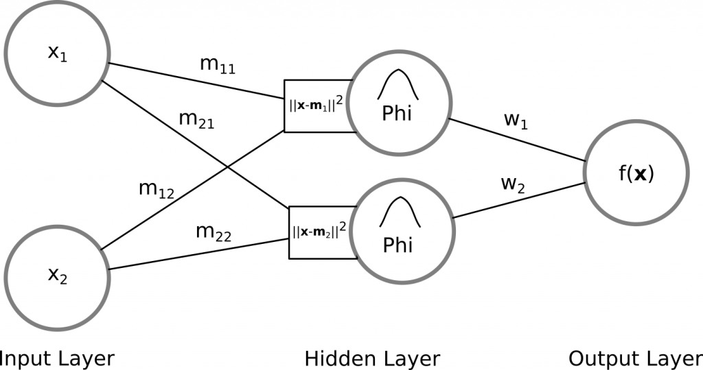
Input to Hidden Layer: Characteristic for RBF networks is the fact that the weights from the input layer to the hidden layer are not what they seem to be as with other ANN. RBF neurons are sometimes called also input weights, protoype vectors or in this case simply centers. Normally one thinks of coefficients which are multiplied with the input neurons in the form of an inner product. But the weights in RBF networks between the input and hidden layer describe rather the position of the RBF neurons in the input space. The activation of a RBF neuron in the hidden layer is then a value/measure of a distance between an input neuron and the rbf neuron and describes how far or how similiar the input neuron is to each of the RBF neurons.

Hidden to Output Layer: The output is the result of a linear combination of the outputs from the RBF functions and their corresponding weights. In other words, a weighted sum is calculated to form the final result.

RBF Networks

Standard form

In the standard formulation a RBF network is defined as the weighted sum of distances between one data point $\mathbf{x}$ and $N$ other inputs $\mathbf{x}_i, i = 1,\ldots,N$ :

$D(\mathbf{o}) = \sum_{i=1}^N \mathbf{w}_i \exp{(-\alpha ||\mathbf{o} - \mathbf{x}_i||^2)}$

Each $\mathbf{x}_i$ (RBF neuron) has a different influence on the data point $\mathbf{x}$ in relation of their position in input space and their corresponding weight $\mathbf{w}_i$ which is affected by $y_i$ as you will see later in the learning phase.

We want to use a RBF network variant that uses only $K$ centers, so we're going to make a slight modification to the formula:

$f(\mathbf{x}) = \sum_{k=1}^K \mathbf{w}_k \phi(\mathbf{r})$

with

$\phi(\mathbf{r}) = \exp{(-\alpha \, \mathbf{r})}$

and

$\mathbf{r} = ||\mathbf{x} - \mathbf{m}_k||^2$

Now we're evaluating a point not with every other point but with every RBF neuron $\mathbf{m}_k$ which represents now a specific center in the data set, with $K \ll N$ . We also generalized the radial basis function by inserting the abstract function $\phi(\cdot)$ . In the following sections other radial basis function will be presented.

The reason for choosing only $K$ RBF neurons is simple: If the standard form is used we will get an exact interpolation. Generally, more RBF neurons result in a more complex decision boundary for solving complex problems. However, the price is payed in computational effort. Even so the goal is to get nearly as good but with less computation involved to evaluate the network.

Before we dive into this, let us check the inner workings of the activation function.

Activation function

Let us first have a detailed look at the radially symmetrical basis function. This function provides the basis for the approximation of our class labels $y_i$ .

$\exp{(-\alpha ||\mathbf{o} - \mathbf{x}_i||^2)}$

The activation function $\phi(\cdot)$ is considered as a distance function with a gaussian distribution. Its centered around $\mathbf{m}_k$ (the mean of the gaussian function is at $\mathbf{m}_k$ ), and has a constant $\alpha$ which is a simplification of $\frac{1}{2\sigma^2}$ :

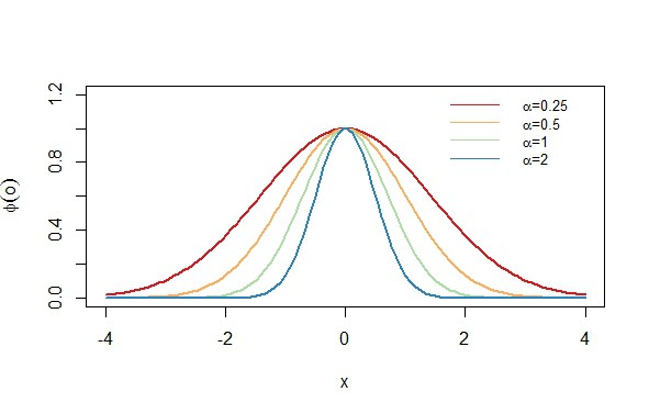
The figure shows a 1-dimensional gaussian function $\phi(x), x=-4,\ldots,4$ with different values for $\alpha$ . The factor $\alpha$ controls the width of the gaussian function as illustrated in the figure. Its centered around 0 because $m=0$ .

Generally speaking, we first calculating the distance of an input neuron (data point) $\mathbf{x}$ with a RBF neuron $\mathbf{m}_k$ according to the euclidean distance $||\mathbf{x}-\mathbf{m}_k||^2$ . The Gaussian then serves as a kind of normalization for the distance measure and expresses the influence of a center on a data point. In conclusion the greater the output of the function the closer the position of a data point $\mathbf{x}$ to the center $\mathbf{m}_k$ . It can also be described as the similarity between two points, so if the distance is minimal ( $\mathbf{r} = 0$ ) the output of that function is maximal ( $\phi=1$ ).

Closer look

First, we generate some data points at random and define our RBF center neuron at $\mathbf{m} = (0,2)$ :

colors <- colorRampPalette(brewer.pal(4,"Spectral"))(4)

m <- c(0,2) # center
x <- cbind(seq(-1,1,length.out = 10), rnorm(10,mean = 2)) # random points

plot(x, pch=16, xlab=expression(x[1]), ylab=expression(x[2]))
points(m[1], m[2],ylim=c(0,3), pch=16, col=colors[1])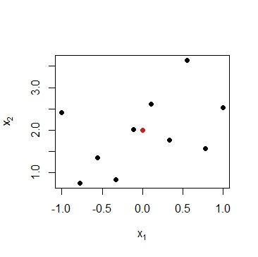

Black points represent 2-dimensional input vectors, and the red dot represents the RBF center neuron

Now we calculate the activation function for each input with the rbf neuron:

# definition of the activation function
activation <- function(m, x, alpha = 1) {  
  exp(-alpha * (sum((x - m)^2)))
}
result <- unlist(lapply(1:nrow(x), function(i) {
  activation(o, x[i,], 1)
}))

Next, we want to check if the neuron with the highest values is truly close to the rbf center and mark it with a green circle in the current plot:

idxMax <- which.max(result) # idxMax = 5
points(x[idxMax , 1], x[idxMax, 2], col="green", cex=2)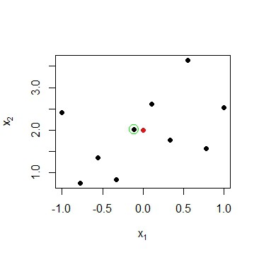

Data point $\mathbf{x}_5$ has an activation of 0.98 in this example and is indeed the nearest neighbour of the rbf neuron.

We can see why that is the case. The output of the radial basis function is affected by the distance: A data point is influenced more by nearby points than by points which are further away. The next figure shows the output of the radial basis function for the rbf center at $\mathbf{m} = (0,2)$ as filled contour lines to see the degree of influence with regard to the distance:

m <- c(0, 2) # rbf center
activation2 <- function(x, y) {  
  exp(-1 * (((x - m[1])^2 + (y - m[2])^2)))
} 

grid <- matrix(rep(seq(-4, 4, by=0.1), 2), ncol=2)z <- outer(grid[,1], grid[,2], activation2)
filled.contour(grid[,1], grid[,2], z = z, xlim=c(-2,3), ylim=c(-1,4), color=colorRampPalette(rev(brewer.pal(4,"Spectral"))))

The figure shows a 2-dimensional shaped "bell-curve"-the symmetry around the center is typical for the gaussian function. The red center of this function depicts the position of the rbf center where the function has a maximum value because the distance is equal to zero.

Other basis functions

In addition to the aforementioned gaussian function it's also possible to use other radial basis function. Here are few examples from this article:

$\phi(r) = r$

$\phi(r) = \frac{1}{1 + \exp{(\frac{{r}}{\sigma^2}-\theta)}}$

$\phi({r}) = {r}^2 \ln{({r})}$

Every function can be used which satisfies $\phi(\mathbf{r}) = \phi(||\mathbf{r}||)$ .

Learning Algorithm

As with any other neural network we have to determine the weights of the RBF neuron. How do we do that? And what other things do we have to learn from the data for the model?

Number of rbf centers
Position of the rbf centers
Weights in the formula
Parameters like $\alpha$ , etc. depends on the actual radial basis function

Selection of RBF neurons

RBF center neurons can be manually selected points from the input data if they're considered to be important, random ones that lie in the same space as the input data or determined by k-means clustering. In each case they should be good representatives of the data set because they affect the classification performance. We don't need the class label for this so it's an unsupervised approach.

Number of RBF centers

It's up to you how many RBF neurons you are choosing. If you're using the k-means clustering approach then you can determine the most suitable cluster size that represents the center points of the data set. See section Improving performance below.

Choosing $\alpha$

The factor $\alpha$ has a very important effect on the performance. The wider the gaussian function the greater the influence on points in the neighbourhood. According to this blog post you can calculate $\alpha$ as follows if you are using k-means clustering for the selection of RBF neurons:

$\alpha = \frac{1}{2\sigma^2}$

where $\sigma^2$ is the mean of data points assigned to a cluster $k$ . So every RBF center neuron gets a different $\alpha$ value assigned. You can also choose one $\alpha$ value for every RBF neuron.

Learning weights

After we selected the centers we can now train the model. We want the following equation to be true for all $N$ data points. we have $N$ equations and $K$ unknowns $\mathbf{m}_k$ because of $K$ centers, and $K \ll N$ . So we have more equations than weights that means we can only approximate $y_i$ :

$\sum_{k=1}^K \mathbf{w}_k \exp{(-\alpha ||\mathbf{x}_i - \mathbf{m}_k||^2)} \approx y_i$

In matrix notation we multiply the $(N\times K)$ -matrix $\boldmath \Phi$ with the $(K \times 1)$ -vector $\mathbf{w}$ to get the $(N \times 1)$ -output vector $\mathbf{y}$ :

$\begin{bmatrix}\exp(-\alpha||\mathbf{x}_1-\mathbf{m}_1||^2) & \cdots & \exp(-\alpha||\mathbf{x}_1-\mathbf{m}_K||^2) \\\exp(-\alpha||\mathbf{x}_2-\mathbf{m}_1||^2) & \cdots & \exp(-\alpha||\mathbf{x}_2-\mathbf{m}_K||^2) \\\vdots & \vdots & \vdots \\\exp(-\alpha||\mathbf{x}_N-\mathbf{m}_1||^2) & \cdots & \exp(-\alpha||\mathbf{x}_N-\mathbf{m}_K||^2) \end{bmatrix}\cdot \begin{bmatrix}w_1 \\ w_2 \\ \vdots \\ w_K\end{bmatrix} \approx \begin{bmatrix}y_1 \\y_2 \\\vdots \\y_N\end{bmatrix}$

$\boldmath \Phi \mathbf{w} \approx \mathbf{y}$

The $i$ $i$ -th row of $\boldmath \Phi$ represents the $i$ -th input neuron; and his estimated output $y_i$ in $\mathbf{y}$ . The $k$ -th weight in $\mathbf{w}$ corresponds to the neuron $\mathbf{m}_k$ in the $k$ -th column of $\boldmath \Phi$ .

We can solve this equation in a linear regression fashion if $\boldmath \Phi^t\boldmath \Phi$ is invertible. The weights can be computed (learned) in one step:

$\mathbf{w} = (\boldmath\Phi^t\boldmath\Phi)^{-1}\boldmath\Phi^t\mathbf{y}$

This should look familiar, and is indeed the least square estimator which is used e.g. in linear regression.

Now you can see the advantage: With only $K$ centers we have to calculate the pseudo-inverse of a $(N\times K)$ -matrix instead of a $(N\times N)$ -matrix.

Because we only get an approximate value for $y_i$ , a real number, we should first rename the new computed class label to $\hat{y}$ . To get things working we need one additional function to get our appropriate class label; the so-called classification function:

$\hat{y} = \lceil \text{signif}(y) \rceil$

where signif is

$\text{round}(10^{-n}\,x)10^{n},\text{ with } n = \lfloor\log_{10}x\rfloor$

Now we're getting natural numbers which is in accordance with our definition of the training set $T$ .

Improving performance

To improve the performance of the rbf model we have to reconsider which parameters of the model can be changed or have to be determined beforehand.

The factor $\alpha$ changes the width of the gaussian function and has a huge effect on the result. When choosing a constant value for $\alpha$ for every rbf center the network may not be fully exploiting its potential if the classes are far apart or a class has a significant higher variance than another class. Then it makes sense to assign or compute an appropriate value for each rbf neuron.

One example for determining $\alpha$ was already shown in the previous section. The easiest way is to select $\alpha$ manually and combine it with the process of cross-validation. Another way is to use a variation of the expectation–maximization algorithm (EM algorithm) to determine one $\alpha$ for all rbf centers or a vector $\boldmath \alpha$ with different values for every center. Have a look at this lecture where it's explained very well.

The number of centers and the position (initial "input weights") also affects the classification performance to a high degree. The number of centers can be calculated and assessed with various methods like the silhoutte or using cross-validation. Still no definitive answer can be given on that problem in general, because the number of clusters in a data set depends on many factors and is very problem-specific. More information on that can be found in this Wikipedia article.

Example in R

To not leave you alone with the theory this section delivers a complete code example that you can go through step by step. For the sake of clarity the R functions were simplified.

activation <- function(o, x, alpha = 0.5) {  
  exp(-alpha * (sum((x - o)^2)))
} 

mysignif <- function(x.iris, p = 1) {  
  n <- floor(log10(x.iris)) + 1 - p  round(10^(-n)*x.iris)*10^n
}

y <- as.numeric(iris[1:100, 5]) # get class labels
x.iris <- iris[1:100, c(1,3)] # get 2d data set of two species
centers <- rbind(c(5, 1.5), c(6, 4), c(5,3.3), c(6.5, 4.7)) # manually define centers

plot(x.iris, col=(y))
points(centers, col="green")

# compute the output of the hidden layer
X <- matrix(0, ncol = nrow(centers), nrow = nrow(x.iris))
for(i in 1:nrow(x.iris)) {  
  for(k in 1:nrow(centers)) {    
    X[i,k] <- activation(centers[k,], x.iris[i,])  
  }
}

# compute weights
w <- solve(t(X)%*%X)%*%t(X)%*%(y)

# check the output
for(i in 1:nrow(x.iris)) {  
  sum <- 0  
  for(k in 1:nrow(centers)) {    
    sum <- sum + w[k,] * activation(centers[k,], x.iris[i,])  
  }  
  points(x.iris[i,], pch=16, cex=0.6, col=(ceiling(signif(sum, 1))))  
  print(paste("for", i, "=", sum, ceiling(signif(sum, 1))))
}

Output image of the script:

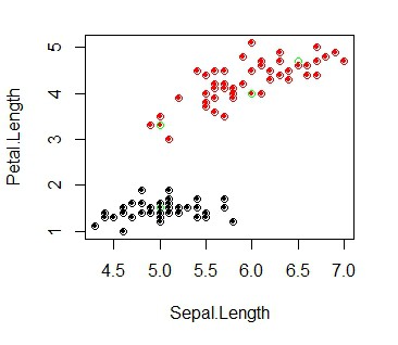
The green points represents the manually selected centers. Three are in the red group and one is in the black group. Here it would make sense to use only 2 centers and assigning different $\alpha$ factors for each. The filled dots depict the calculated output where the coulered circles show the actual data point for each class. In this example all output labels were computed correctly. Now you have your RBF network classifier!

References

Lecture of the Caltech's Machine Learning Course - CS 156 by Professor Yaser Abu-Mostafa about radial basis functions
https://www.youtube.com/watch?v=O8CfrnOPtLc
Great article about rbf networks with MATLAB code example
https://chrisjmccormick.wordpress.com/2013/08/15/radial-basis-function-network-rbfn-tutorial/
Definition of the signif function
https://en.wikipedia.org/wiki/Significant_figures
Paper "Using Radial Basis Function Networks for Function Approximation and Classification"
http://www.hindawi.com/journals/isrn/2012/324194/

Dominik Grzelak blog

Radial Basis Function Networks (RBFN) for Classification with k Centers