Introduction
This article provides a brief introduction for a special subject in a typical data mining process: data normalization. Most of the time, after you collected your data, visualized it and computed some statistical values, you have to pre-process the data at one point. Normalization falls within the field of preprocessing which also includes:
- Feature extraction
- Feature reduction
- Feature selection
Data normalization is not to be confused with the above mentioned topics.
Normalization methods will not make new features nor select optimal features.
More precisely normalization belongs to the field of data transformations. Transformation includes techniques such as binning, smoothing, aggregation, etc. In literature the term standardizing and normalization have slightly different meanings but I will use both interchangeably.
The first part will answer the question why it's sometimes useful to normalize data before applying modelling methods. In the second part I will outline some of the most common methods how to scale numerical values. As far as my understanding goes, scaling of categorical variables falls into the category data transformation in general and will not be discussed here. It's rather a mapping of factor levels into a set of values. For the practical part of this articles I provide examples and R code snippets to follow along the explanations.
Why I have to normalize my data?
The main reason for normalizing features of a dataset is to ensure that attributes can be compared among each other. Normalization will give you a standardized dataset. This consequence is closely connected with the points listed below:
- Comparable Features
- Improved Classification Accuracy
- Faster Learning
- Improved Features
Keep in mind that normalization will not automatically give you all the advantages listed here. As in all data mining tasks the method depends on the actual problem and of course which classification or prediction model is being used.
An example: If you do handwriting detection and you're not normalizing your input data then your neural network will have a hard time to predict the correct outcome. Technically there're endless possibilities how a letter could be introduced to the network:
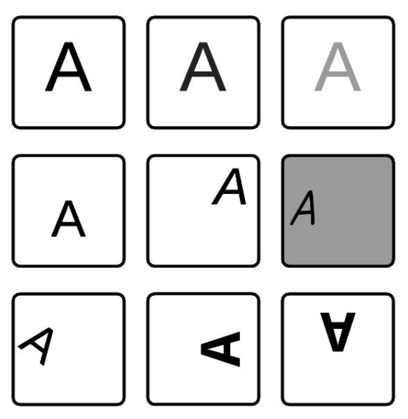 Normalization in that example means to unify the intensity of the image (brightness, contrast), the size or position (translation, rotation, disposition) etc. If no transformation is performed a network might have problems to learn all these different kind of training samples although they belong the same class. It doesn't mean that this is an impossible task but a standardized dataset will result in shorter learning time and in a better performing classificator.
Comparable Features
Normally a dataset contains of different kinds of features whereby values can have uneven value ranges if compared to each other. I don't mean outliers in that sense but merely features that have a large range e.g. income in comparison to age. Or attributes that aren't normally distributed but rather log-normal distributed which is very common in the geological, biological or medical domain. Such features will be attributed with high relevance, and outweighing others with smaller value ranges. Data transformation can help us to bring all features in a common range to give each feature the same importance-in other words, to make them comparable.
Imagine you have a dataset with an attribute in percentage and a numerical one like GDP of a country which has a much larger value range and therefore a higher influence on the distance calculated if e.g. k-Nearest-Neighbour is applied. This advantage of normalization is closely connected to the second one described below ("Improved Classification Accuracy"). That is also true if you want to compare numerical and categorical variables.
An example shall illustrate that problem and is inspired from this blog post. Imagine you have this very small income dataset and one would like to find similar pairs.
| ID | Income | Age |
| 1 | 45000 | 45 |
| 2 | 43000 | 30 |
| 3 | 8000 | 17 |
| 4 | 41000 | 42 |
To compute the similarity between two entries we can use the euclidean distance. The results are shown in the distance matrix below where the distance for every possible combination between two observations were calculated:
| 1 | 2 | 3 | |
| 2 | 2000.056 | 0 | |
| 3 | 37000.011 | 35000.002 | 0 |
| 4 | 4000.001 | 2000.036 | 33000.009 |
The smaller the value the similar two observations are. The distance between one entry with itself is zero and is shown in the diagonal of the matrix. You can clearly see that the entries with ID 1 and 2 are very similar in contrast to 1 and 4. But there is one problem: The difference between the income of entry 1 and 2 is: |4500 - 43000| = 2000. This is nearly the same as the distance measure has returned d(1,2) = 2000.056. That means that the feature income has a much higher importance than feature age and doesn't count much in the similarity calculation as income, which is dominating the calculation. From the dataset we would expect that 1 and 4 are more similar than 1 and 2.
This approach is used for example in the k-Nearest-Neighbour Algorithm and you can see that the algorithm would benefit from normalization as presented in here, there or here.
Sometimes the counterpart is necessary. It may be possible that the features should retain their different importance/weight so you have to think about which normalization method you are applying.
Improved Classification Accuracy
Some of the classification models require input values within a specific range. Consider for instance neural networks---most of them require a range of [0,1] or [-1,1] to work properly [pyle1999data].
But there is no explicit requirement that the input data has to be normalized but can have a positive effect in the learning phase. For MLP it is also even better to scale between [-1,1] (or [-5,5] etc.) than [0,1], in fact any interval so that the center of the data is 0, c.f. ftp://ftp.sas.com/pub/neural/FAQ2.html#A_std.
That is also true for categorical variables that have to be transformed into numerical or binary ones, e.\,g. two classes as {0,1} or {-1,1} for SVM. But that is rather the topic of data transformation than normalization and I therefore will not further discuss it here. Have a look at this book [pyle1999data].
Especially for distance measures, which are involved in many classification methods like kNN or RBF Networks, normalization can have a huge impact on the classification accuracy and can improve it tremendously. See an example in this paper where the parkinson dataset of the UCI machine learning repository was used in connection with a K-nearest Neighbor Algorithm for classification. Different normalization methods where applied to measure the effect on the correct classification rate. It was pointed out that a scaled dataset achieved a better performance than an unscaled one.
Faster learning
A normally distributed dataset will "reduces numerical difficulties related to MLP and SVM learning algorithms" [holmes2011data].
Especially neural networks trained with the backpropagation algorithm can benefit from normalized features. Again the scaling method depends on the training algorithm that is applied. Neural networks with standard backpropagation algorithm (uses the gradient descent approach) is very sensitive to normalization and can lead to slow convergence of the training, see ftp://ftp.sas.com/pub/neural/FAQ2.html#A_std. A normalization within [-1,1] will generally result in a shorter learning time.
"Improved" Features
Normalization is very common in digital image processing when it comes e.g. to correct the brightness level of an image. This falls under the category of distribution normalization which will not be further addressed in this article but I felt that it has to be mentioned here for the sake of completeness. For example take this gray scaled picture on the left hand side:
 |
 |
Picture of a cat in grayscale, Plot of the histogram for the grayscale image
The right image shows a plot of a histogram and visualizes the distribution of the pixel values (ranging from 0 to 1) from the left image. The kernel density estimate with a Gaussian kernel is added as well.
library(jpeg)
img <- readJPEG("cat.jpg")
hist(img, freq = F, ylim=c(0, 15), ylab="relative frequency", xlab="gray scale value", main="")
lines(density(img))
We clearly see a skewed right distribution. Only a a small amount of the whole gray scale range is covered in the picture. There are more darker pixels in the picture than brighter ones. Very bright shade of colours are not present (no bar above 0.75). But we also conclude from the distribution that the background (the meadow) is still "bright": the tail of the distribution is long and not zero until it reaches ; not the majority of the pixels but they're still there! If the distribution would be normalize than the image would be much brighter. So "improved" features in this case means more balanced lighting conditions for the image.
Methods
Min-Max Normalization
The best known normalization technique is the Min-Max normalization method which scales individual values between the range :
|
|
, |
where is the
sample of the vector
; and
the normalized value. We can extend this formula the scale a feature between a specific interval
:
|
|
R Code Snippet The following R code shows a function which scales the column vectors (the features) of a whole data.frame or matrix:
minmax <- function(m) {
idx <- 1:ncol(m)
mins <- sapply(m[,idx], min)
maxs <- sapply(m[,idx], max)
b <- maxs - mins
sapply(idx, function(i) {
(m[,i] - mins[i]) / b[i]
})
}
Closer look Regarding the reasons for normalization have a look at this example. A dataset with three different attributes x, y and z are
randomly generated and follow a normal distribution with different means and standard deviations:
data <- data.frame(x = rnorm(10), y = rnorm(10, 10, 4), z = rnorm(10, 20, 2))
data.scaled <- minmax(data)
If you would calculate the distance between those points in the three dimensional space then attribute will outrank the other two attributes in the distance calculation so that the points can't really compared with each other. Min-max normalization solves the problem of comparability. The illustrative result is presented in the following table:
| x | y | z | |
| Before Normalization | |||
|
|
1.16 | 15.46 | 15.18 |
|
|
-0.06 | 21.64 | 15.36 |
| After Normalization | |||
|
|
0.38 | 0.29 | 0.30 |
|
|
0.52 | 0.49 | 0.44 |
After normalization all features will approximately have the same mean and variance which makes same equally important.
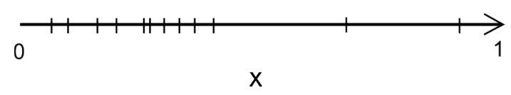
Problems with this normalization method This method has the property, that points in the input space will be almost normally distributed:
 But if extreme outliers are present in the dataset then the scaled values are getting skewed to one side which is not optimal:
 Outliers remain a problem as before so you have to eliminate them beforehand.
z-Score Normalization
Also know as standard deviation normalization, where the mean and standard deviation of each feature is calculated from the dataset and a sample of a feature vector
is transformed as follows:
|
|
where is the standard deviation for the feature vector
; and
the mean. This method is applied to individual values.
The property of this scaling method is that your data will be normally distributed with and
and is different from the Min-Max method where those values vary depending on the interval
used for scaling:
This method is appropriate for outliers in the dataset and they will not affect the transformation. So it makes it favourable to the Min-Max normalization in some cases.
R Code Snippet
zscore <- function(m) {
idx <- 1:ncol(m)
means <- colMeans(m)
sds <- sapply(m[,idx], sd)
sapply(idx, function(i) {
(m[,i] - means[i]) / sds[i]
})
}
Example In this example we use the trees dataset from within the R environment and using the height attribute for scaling:
> trees$Height
[1] 70 65 63 72 81 83 66 75 80 75 79 76 76 69 75 74 85 86 71 64 78 80 74 72 77 81 82 80 80 80 87
> mu  sigma  (trees Height - mu) / sigma
[1] -0.9416472 -1.7263533 -2.0402357 -0.6277648  0.7847060  1.0985884 -1.5694121 -0.1569412  0.6277648 -0.1569412 ...
You can check by yourself if the normalized values fulfil the properties mentioned above
Decimal scaling
This method is moving the decimal point of the values that each value falls into a range between :
|
|
where is the smallest integer such that
.
Example Imagine a vector with range
. Let
be 32. First, we have to find the value with the largest magnitude, in this case it would be -455. Then we would scale this value to -0.455 by dividing it by 1000. So
is 3 in this example and the above condition is met
. Therefore the value
would be transformed to
.
Max Scaling
Each value is normalized by dividing it by the maximum of the feature variable
:
|
|
All normalized values will fall in a range between .
Logarithmic scaling
Log transformation for a value is computed as follows:
|
|
ith base . If the data has a highly skewed distribution it advisable to use this scaling method to reduces the skew in the data, or in other words to "linearise" it. Thus making possible relationships in the data more interpretable.
It's commonly used in regression, which the following example also shows. We're using the Forestfire Data Set from the UCI machine learning repository.
The attribute area, describing the burned area of the forest (in ha), has a right skewed distribution if we look at the histogram. We're only looking at a subset of the data at the moment by selecting only those entries that fall into the month august and have a burned area greater than zero.
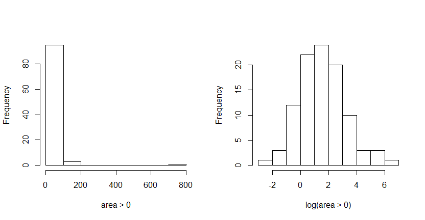
It makes sense to log transform the data which is depicted in the right histogram of this figure. It's a really nice log-normal distributed set now!
For the non transformed data you couldn't exactly say what the largest burnt down area was in august. The highest proportion of the burned area is between 0 and 100 ha. This may give you a false perception and inaccurate description of the data whereby the log transformed data is easier to interpret. The highest proportion of the burned area lies between 1 and 2, that means between 2.72 and 7.39 ha. To get the pre-transformed values you have to inverse the transformation, and in this case it would be .
Closer look This transformation makes skewed or wide distributions easier to read which is the case with most monetary data like income, salaries, purchase size or values without any units like percentages. The same applies to logistic growth processes of yeast strains or other organic growth processes.
The main disadvantage of this method is that it cannot be applied for negative values or zeros. There are several variations for this scaling method, for example the,
, or the signed log transformation, as explained in this blog post. You can also find further explanations when to log transform your data.
Whitening
This method will decorrelate the dataset. Correlated data points to the fact that features may not be independent from each other. It means that a change in attribute A will affect attribute B in some sense. The higher the correlation the larger the effect in change. Highly correlated features may be considered as redundant because the tend to favour the same information.
To avoid this we can use the whitening approach where all values are transformed with mean of 0, variance 1 and covariance 0:
|
|
where is the mean vector of a
matrix
; and
the
sample of
; and
is the diagonal matrix of eigenvalues of the covariance matrix of
; and
the matrix composed of eigenvectors corresponding to
. This method is slightly different from the others. While the others are applied to each individual value of a feature this method is applied at once on all features of an observation.
R Code Snippet
C <- cov(X)
e <- eigen(C)
o <- order(e$values, decreasing=F)
lambda <- diag(e$values[o])
U <- e$vectors[,o]

mu <- colMeans(X)
M <- matrix(rep(mu, 50), ncol=2, byrow=T);
xt <- t((sqrt(solve(lambda))%*%U)%*%t(X-M))
Closer look We begin by generating a correlated dataset with different mean and standard deviations and plotting the two features against each other:
X <- cbind(rnorm(40,1), rnorm(40,1)*9+13);
plot(X[,1], X[,2]);

cov(xt)
colMeans(xt)
plot(xt[,1], xt[,2])
We can observe that the mean of matrix xt is now 0 and all covariances disappeared. The the difference in the non-normalized dataset and the normalized one:
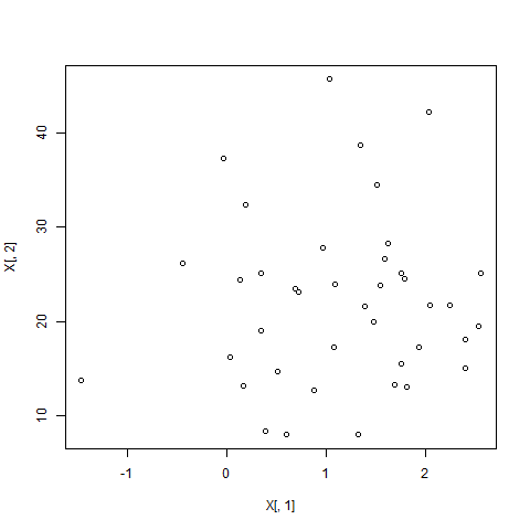 |
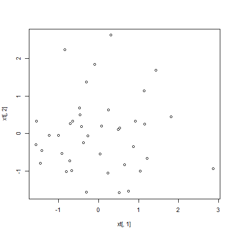 |
Left: Date before normalization, Right: Data after whitening applied
Summary
The table below shows a summary of the value range and characteristic properties of the scaled data for all mentioned normalization methods.
| Method |
|
|
|
|
|
| Min-Max-Normalization | x | x | x | ||
| zScore-Normalization | x | ||||
| Log-Normalization | x | ||||
| Maximum-Normalization | x | ||||
| Decimal-Normalization | x | ||||
| Whitening | x |
Remember
- It's important to store the parameters that were involved during the normalization. If a predictor gets a good result on a normalized data set than you want to scale new data in the same way. Otherwise you get a different transformed dataset which may give you other results. The stored parameters depending on the method and might be the mean, the interval boundaries, maximum value etc.
- Use z-Score normalization or Min-Max normalization with a value range of
for neural networks trained with backprop (other learning algorithms may be scale invariant so you don't need scaling).
- Scale features to make them comparable among each other if a) you're using distance measures, and b) the scale of the attributes is not meaningful.
- Use log transformation with data that have a very wide distribution or are highly skewed.
References
[pyle1999data] Data Preparation for Data Mining, Pyle, D., 1999
[holmes2011data] Data Mining: Foundations and Intelligent Paradigms: VOLUME 2: Statistical, Bayesian, Time Series and other Theoretical Aspects, Holmes, D.E. and Jain, L.C., 2011